What better way to learn than to do? I decided to implement from scratch some Machine Learning algorithms I’m learning as a way to better understand and internalize them. The algorithms include Linear Regression, K Nearest Neighbors, Support Vector Machine, Naive Bayes, K Means and Neural Networks.

ML Chops is a series meant to explain the inner workings of these algorithms so you can get a pretty good grasp of how they work as well as know how to implement them yourself. We’ll be using the Python programming language.
There’s a repo on my GitHub where all the code can be found. The url is: https://github.com/nicholaskajoh/ML_Chops.
The ML Chops series
- Linear Regression (this article)
- K Nearest Neighbors
- Naive Bayes
- Support Vector Machine
- K Means
Machine Learning
I’m assuming the term Machine Learning is not strange to you. You may not really know how to implement or use Machine Learning algorithms, but you probably have some intuition about how it all works. You essentially “train” an algorithm/a model with data and then it’s able to make predictions, a lot of times very accurately.
If all this sounds like Mandarin, you should probably watch Josh Gordon’s explanation of what Machine Learning is.
If you’re good at this point, then let’s talk Linear Regression.
Linear Regression (LR)
Linear Regression is a simple model for predicting continuous data/real-valued outputs. It’s commonly used in subjects like physics, chemistry and math. I first came across it in secondary school practical physics when I had to predict outputs using data recorded during experiments. Sound familiar? 🙄
Imagine you want to predict the price per barrel of crude oil in Nigeria for tomorrow, next week or next month. With data on the prices over the years or past months, you can make a fairly accurate forecast of what the price would be using LR. Keep in mind that we’re assuming the data is correlated (positively or negatively). If it’s not correlated, then LR is probably not a good fit. We’ll talk about other algorithms that can handle nonlinear data later on in the series. For now we need to use linear data else, our predictions would be really really bad. We don’t want bad! 😒
The graph below may help you visualize linear data better…
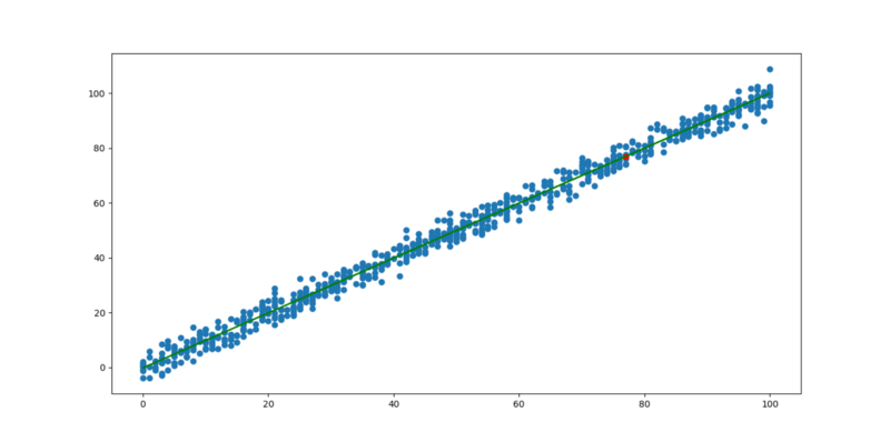
Graph of linear data
The first thing you probably noticed is how somewhat scattered the data points are. There’s a pattern though, and it’s linear. As the value on the horizontal axis increases, the value on the vertical axis [generally] increases as well (positive correlation).
Best fit line
There’s a green line that passes through some of the points on the graph. It’s called the line of best fit. Ideally this line should pass through all the points. However there is some “error” in the data. This explains why there is some scatteredness in the plot.
The line of best fit is the best possible line you can draw to fit the data. If the data had no errors, this line would pass through every point in the graph. The real world is not that perfect though. There’s always some degree of error. For instance, the price of crude oil generally increases year after year but not by a constant amount. It may increase $3 this year and $1 next year. As a result, we can’t know for sure how much it would cost in the near future, but we can make predictions given the best fit line. But how do we get the best fit line?
Equation of a line
Recall the equation of a straight line? It’s y = mx + c. The best fit line is a straight line so we can use this equation to figure it out.
x is the independent variable. In the case of the crude oil example, it’s a year (e.g 2001, 2002, 2003, …, 2010 etc).
y is the dependent variable. This is the value we want to predict. Given the prices of oil from 2001 to 2010, we may want to predict the price in 2011, 2012 or even 2018.
m is the slope of the line. It’s a number that measures its “steepness”. In other words, it is the change in y for a unit change in x along the line.
c is the y intercept. That is, the point where the line crosses the vertical/y-axis.
We know x. We want to find y. We just need to figure out what m and c is for the best fit line (of a given data set) to be able to make predictions… 🤔
It turns out that there are formulas from which we can evaluate the slope, m and y intercept, c. Once we get the slope and y intercept, our model is ready!
Mathematically, our LR model may look like this: y = 2.1x + 1.4 where m = 2.1 and c = 1.4
Slope
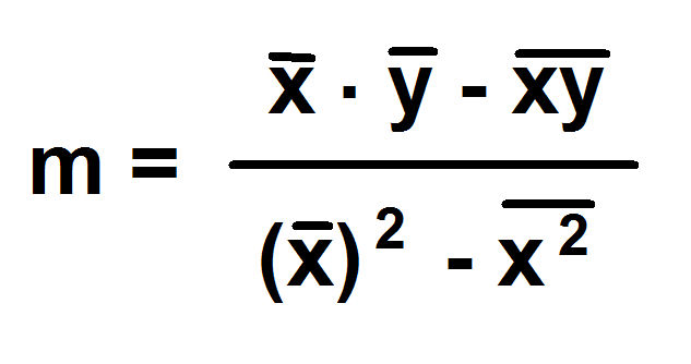
slope formula
NB: the bar symbol represents mean/average. E.g “X bar” is the mean of the Xs in the dataset.
Intercept
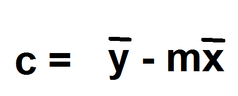
y intercept formula
Simple example
Say we have the years 2001, 2002, 2003, …, 2010 and oil prices 43.1, 45.2, 43.7, 49.0, 50.5, 53.7, 53.0, 56.8, 57.2, 60.0. We could come up with a table like so:
x (yrs)   1    2    3    4    5    6    7    8    9    10

y (in $)  43.1 45.2 43.7 49.0 50.5 53.7 53.0 56.8 57.2 60.0
I used 1 to 10 to represent 2001 to 2010 so that calculations would be easier to comprehend. It doesn’t affect anything. You can use the years to do your calculation if that resonates with you. Keep in mind though that the difference of any two consecutive values of x must be 1.
Using code, we can calculate the slope and intercept like so:
import numpy as np
from statistics import mean

xs = np.array([1, 2, 3, 4, 5, 6, 7, 8, 9, 10])
ys = np.array([43.1, 45.2, 43.7, 49.0, 50.5, 53.7, 53.0, 56.8, 57.2, 60.0])

m = ((mean(xs) * mean(ys)) - mean(xs * ys)) / (mean(xs)**2 - mean(xs * xs))

c = mean(ys) - (m * mean(xs))
Predict
If we want to predict how much oil would cost in 2018, all we need to do is supply x in our model. x would be 18. Thus:
x = 18
y = m * x + c
print(y)
Model accuracy
Accuracy is very important to Machine Learning developers. Our LR model makes predictions. It’s of interest to us to know how accurate these predictions are. While 80% accuracy of a model that predicts the price of oil for me sounds good enough, it’s probably a deal breaker for my client who buys and sells oil. He’s probably looking for somewhere around 95 to 99.9%. 80% is too much risk!
There are several ways to calculate how accurate a LR model is. We’re going to talk about one of them called R-squared. It’s a statistical measure of how close the data are to the fitted regression line/best fit line. It is also known as the coefficient of determination. With R-squared, we’re simply asking: how good is the best fit line?
Of course, if the best fit line is not good enough, then it’s the data to blame (it’s the best fit line duh 😜). Regardless, it means the predictions made using the line would be less accurate.
R-squared is given by the formula:
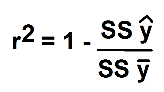
r squared
SS stands for Sum of Squared error of
y hat line (y with the caret) is the ys of the best fit line ( for each x)
y bar is the mean of the ys
To calculate the R-squared for a given model:
best_fit_line = [(m * x) + c for x in xs]

SSy_hat = sum([y * y for y in (best_fit_line - ys)]) # y hat line
SSy_mean = sum([y * y for y in [y - mean(ys) for y in ys]]) # mean of ys

r2 = 1 - (SSy_hat / SSy_mean)
The range of r2 is usually 0 to 1 so you can multiply it by 100 to get a percentage.
Don’t forget to check out the repo for the complete Linear Regression code: https://github.com/nicholaskajoh/ML_Chops/tree/master/linear-regression.
If you have any questions, concerns or suggestions, don’t hesitate to comment! 👍
Last modified on 2023-03-14