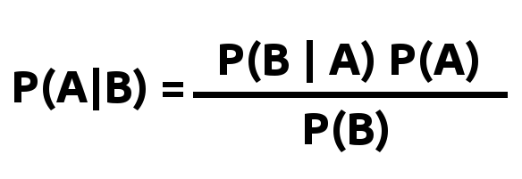
Naive Bayes is a classifier just like K Nearest Neighbors. The Naive Bayes algorithm applies the popular Bayes Theorem (used to calculate conditional probability) given by the formula:

Bayes formula

Here’s a great explanation to read if you’ve not come across/don’t understand the theorem yet: https://betterexplained.com/articles/an-intuitive-and-short-explanation-of-bayes-theorem.

The ML Chops series

Let’s consider the data we used in the last post on KNNs:

height (ft)    weight (kg)    sex  
6.3            50.2           Male  
5.9            79.7           Female  
5.1            61.4           Female  
5.6            47.1           Male  
5.1            59.8           Female

In Naive Bayes, we calculate the probabilities of an input feature set being in each of the classes in the data and return the class with the highest probability as the predicted output.

Our goal with the data in the table above is to determine whether an individual is Male or Female. Given the height and weight of a person e.g [height, weight] -> [5.8, 82.1], a Naive Bayes classifier calculates the probabilities of the person being a Male and a Female e.g [(“Male”, 7.92248128417e-103), (“Female”, 0.00355626444241)] then returns the class with the highest probability (in this example “Female”).

How do we find the probabilities for each class?

You guessed right! Bayes formula.

Let’s put the formula into context for better understanding:

Probability that a person is Male

Substitute Female for Male in the formula and you have the probability that a person is female.

Let’s explain terms in the equation briefly:

P(Male | height & weight) is the probability that a person is Male given their height and weight (better put: given all the features provided in the data). This is what we’re looking for.
P(Male) is the probability of selecting a Male person from the data.
P(height | Male) and P(weight | Male) equate to P(B|A) [from the first formula]. P(height | Male) is the probability of getting the height of a person given that they are Male (same for the weight). Essentially we want to find the percentage of Males with the same height as the person we’re classifying. This not feasible with our data however because both height and weight are continuous. Besides, it would be very costly when we have a large amount of training data (we’d have to run through the data every time to count the number of people with same height and weight with the person being classified). Thankfully, we have the Probability Density Function (PDF) to help us with this. We’ll use PDF to determine both P(height | Male) and P(weight | Male) in a bit.
P(height & weight) or better put P(all features) is the marginal probability. For our classification, it’s not really useful to us because it’s the denominator for all class probabilities. We’re actually interested in finding the class with the highest probability and not the actually probability figure like 0.9 for instance. We might as well not use it since we’re dividing by it in every class probability calculation. It doesn’t change anything. We’ll still get the class with the highest probability.

P(Class)

The probability of selecting a person from a given class is the simplest calculation to perform. From the data table, we can see that there are 5 samples. 2 are Male. Thus P(Male) = 2/5. And 3 are Female. Thus P(Female) = 3/5.

The PDF

The PDF can be computed using the following formula:

The PDF

Substitute Female with Male and/or weight with height to calculate other PDFs.

Using PDF, we assume:

Each feature is uncorrelated from the others (i.e height is independent of weight for instance).
The values of the features (i.e heights, weights) are normally distributed.

These are assumptions and are not completely true most times for a given data set. As such, we’re being “naive” by assuming.

Code

First things first! The data.

For convenience, I’m using 3 arrays:

import numpy as np

# data  
heights = np.array([6.3, 5.9, 5.1, 5.6, 5.1])  
weights = np.array([50.2, 79.7, 61.4, 47.1, 59.8])  
classes = np.array(["Male", "Female", "Female" , "Male", "Female"])

Next, let’s find P(Class) for Male and Female:

males_count = 0  
females_count = 0  
sample_size = len(classes)  
for x in classes:  
    if x == "Male":  
        males_count += 1  
    else:  
        females_count += 1  
p_male = males_count / sample_size  
p_female = females_count / sample_size

PDFs

We need to find the various means and variances required to compute the PDFs:

heights_of_males = []  
weights_of_males = []  
heights_of_females = []  
weights_of_females = []

for i in range(sample_size):  
    if classes[i] == "Male":  
        heights_of_males.append(heights[i])  
        weights_of_males.append(weights[i])  
    else:
        heights_of_females.append(heights[i])  
        weights_of_females.append(weights[i])

mean_height_males = np.mean(heights_of_males)  
mean_weight_males = np.mean(weights_of_males)  
mean_height_females = np.mean(heights_of_females)  
mean_weight_females = np.mean(weights_of_females)  
var_height_males = np.var(heights_of_males)  
var_weight_males = np.var(weights_of_males)  
var_height_females = np.var(heights_of_females)  
var_weight_females = np.var(weights_of_females)

Now to the PDF formula in code…

Let’s define a function as we’ll use it severally:

def the_pdf(x, mean, variance):  
    pd = 1 / (np.sqrt(2 * np.pi * variance)) * np.exp((-(x - mean)**2) / (2 * variance))  
    return pd

Predict

x = [5.8, 82.1] # [height, weight]

p_height_male = the_pdf(x[0], mean_height_males, var_height_males)
p_weight_male = the_pdf(x[1], mean_weight_males, var_weight_males)
p_height_female = the_pdf(x[0], mean_height_females, var_height_females)
p_weight_female = the_pdf(x[1], mean_weight_females, var_weight_females)


# Get class probabilities  
p_male_h_and_w = p_male * p_height_male * p_weight_male  
p_female_h_and_w = p_female * p_height_female * p_weight_female  
print("P(Male | height & weight) =", p_male_h_and_w)  
print("P(Female | height & weight) =", p_female_h_and_w)

# Return prediction  
if p_male_h_and_w > p_female_h_and_w:  
    print("class = Male")  
else:  
    print("class = Female")

Output:

P(Male | height & weight) = 7.92248128417e-103  
P(Female | height & weight) = 0.00355626444241  
class = Female

Putting everything together, we have:

Don’t forget to check out the ML Chops repo for a more robust and efficient implementation: https://github.com/nicholaskajoh/ML_Chops/tree/master/naive-bayes.

If you have any questions, concerns or suggestions, don’t hesitate to comment! 👍

Last modified on 2023-03-14