The Support Vector Machine (SVM) is a supervised learning model used for classification and regression. In this tutorial, we’ll be using it for classification.

The ML Chops series

Linear Regression
K Nearest Neighbors
Naive Bayes
Support Vector Machine (this article)
K Means

Created by Vladimir Vapnik in the 1960s, the SVM is one of most popular machine learning classifiers. Given a set of training samples, each marked as belonging to one or the other of two categories, the goal of SVM is to find the best splitting boundary between the data. This boundary is known as a hyperplane — the best separating hyperplane.

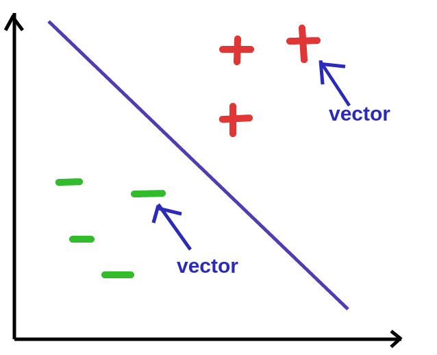
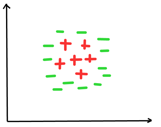
Let’s take the points on the graph below for example:

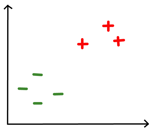
What line best divides the red pluses and green minuses? Eye-balling the data points, I came up with this.

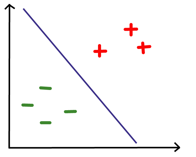
Any data point that falls on the right side of the boundary is classified as a red plus and any point that falls on the left side is classified as a green minus.

How do we arrive at the best separating hyperplane, mathematically?

Well, the equation of a hyperplane is given by wx + b = y where w is the normal vector to the hyperplane, b is a bias/shift and x is a vector the hyperplane passes through. y determines the position of the hyperplane.

Take a look at the diagram below for better understanding:

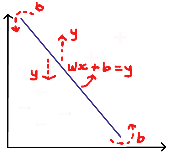
It turns out that y = 0 at the best separating hyperplane. Thus the equation of the best separating hyperplane is wx + b = 0.

With this hyperplane, it shouldn’t be difficult to determine if an input vector (a feature set we desire to classify) is on one or the other side of it. To make a prediction, we’d return the sign of wx + b. A positive sign (+) represents one class and negative sign (-) represents the other.

There’s just one problem. We need to find w and b when y = 0. Now there’s a new question to answer. How do we find w and b?

We’ll come to that in a bit.

What are Support Vectors?

In SVM, each sample in a data set is a vector. The area covered by the data points is a vector space.

A support vector is a vector in this vector space which determines the hyperplane that best separates the data. They are the closest points to the best separating hyperplane.

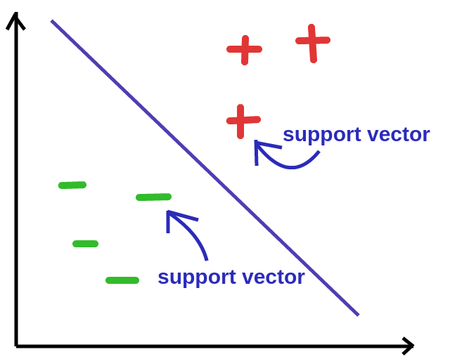
If any of the support vectors change, the best separating hyperplane changes as well. You could say they “support” the best separating hyperplane.

We can draw 2 hyperplanes both parallel to the best separating hyperplane that pass through the support vectors. The best separating hyperplane divides these hyperplanes into two equal parts/areas.

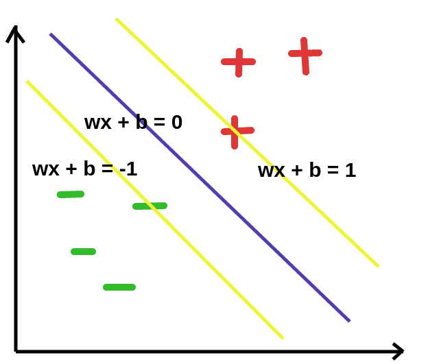
It turns out that these two hyperplanes are given by wx + b = -1 and wx + b = 1 as show in the graph above.

w and b

The geometric distance between the hyperplanes enclosing the best separating hyperplane is 2 / ||w|| where ||w|| is the magnitude of w.

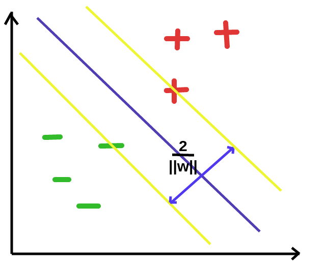
This distance is maximum at the values of w and b which produce the best separating hyperplane. As such, our goal is to get a value of w and b that maximize 2 / ||w||. Maximizing 2 / ||w|| equates to minimizing ||w||, so we could as well do just that.

For mathematical convenience, let’s minimize 1/2 * ||w||² instead of ||w||. Note that this doesn’t change anything. Minimizing ||w|| is minimizing 1/2 * ||w||².

There’s a constraint to this minimization given by y(wx + b) >= 1. This ensures that we don’t maximize the distance beyond the 2 hyperplanes that separate the 2 categories of data.

This is a classic quadratic optimization problem!

We are tasked with minimizing 1/2 * ||w||² subject to y(wx + b) >= 1.

There are several methods for optimization at our disposal including Convex Optimization and the popular Sequential Minimal Optimization (SMO) invented by John Platt in 1998 at Microsoft.

We’ll be using Convex Optimization to solve this problem.

Convex Optimization

I chose to use the CVXOPT python library for Convex Optimization because I didn’t want to delve into too much math. Feel free to explore Convex Optimization (the math and the code). Here’s a little explanation of convex optimization for the problem we’re solving — to get optimum values of w and b.

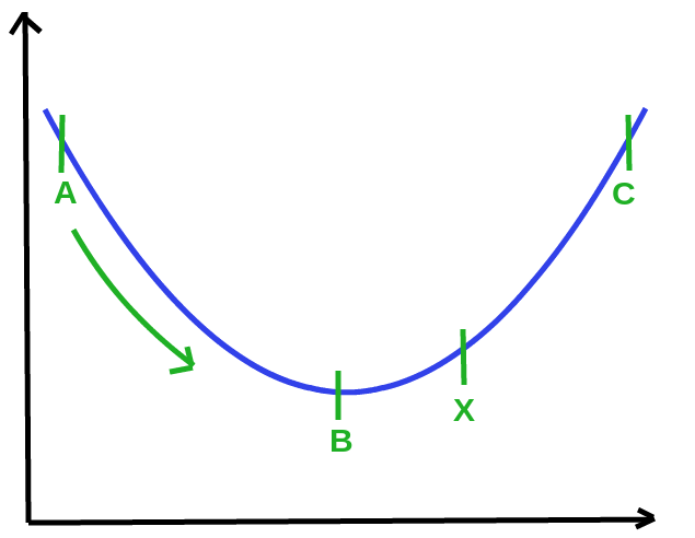
Suppose the optimum value for w and b is at X. We could move from A to C in a bid to get to X. B is the point where 1/2 * ||w||² is minimum but it does not satisfy the constraint y(wx + b) >= 1 (in this example) so it’s not the optimum point.

Code

Data:

import numpy as np  
import cvxopt  
import cvxopt.solvers

features = np.array([[5, 4], [5, -1], [3, 3], [7, 9], [6, 7], [7, 11]])  
labels = np.array([-1.0, -1.0, -1.0, 1.0, 1.0, 1.0])

Train/fit using CVXOPT:

def fit(X, y):  
  n_samples, n_features = X.shape

  # Gram matrix
  K = np.zeros((n_samples, n_samples))  
  for i in range(n_samples):  
    for j in range(n_samples):  
      K[i,j] = np.dot(X[i], X[j])

  P = cvxopt.matrix(np.outer(y,y) * K)  
  q = cvxopt.matrix(np.ones(n_samples) * -1)  
  A = cvxopt.matrix(y, (1, n_samples))  
  b = cvxopt.matrix(0.0)  
  G = cvxopt.matrix(np.diag(np.ones(n_samples) * -1))  
  h = cvxopt.matrix(np.zeros(n_samples))

  # solve QP problem
  solution = cvxopt.solvers.qp(P, q, G, h, A, b)

  # Lagrange multipliers
  a = np.ravel(solution['x'])

  # Support vectors have non zero lagrange multipliers
  sv = a > 1e-5  
  ind = np.arange(len(a))[sv]  
  a = a[sv]  
  sv_ = X[sv]  
  sv_y = y[sv]

  # Intercept
  b = 0  
  for n in range(len(a)):  
    b += sv_y[n]  
    b -= np.sum(a * sv_y * K[ind[n], sv])  
  b /= len(a)

  # Weight vector
  w = np.zeros(n_features)  
  for n in range(len(a)):  
    w += a[n] * sv_y[n] * sv_[n]

  return w, b

Predict:

w, b = fit(features, labels)

def predict(x):  
  classification = np.sign(np.dot(x, w) + b)  
  return classification

# test  
x = [3, 4]  
print(predict(x))

The Kernel trick

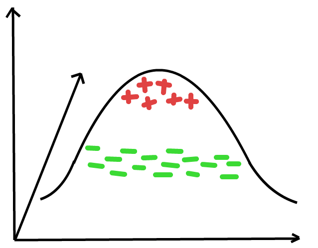
The data we’ve been dealing with is linearly separable i.e we can draw a straight line (speaking in 2D) that separates the data into 2 categories. What if we have a data set like this?

There’s no hyperplane that can separate this data.

The kernel trick introduces a new dimension to the vector space. Adding a dimension to the data in the diagram above yields a 3D vector space. Can we separate the data now? Probably.

If we can’t we could add more dimensions until we can. That’s beyond the scope of this tutorial so we won’t go any further. Do read about kernels in SVM though. There’s some pretty interesting stuff to explore!

Don’t forget to check out the ML Chops repo for all the code: https://github.com/nicholaskajoh/ML_Chops/tree/master/support-vector-machine.

If you have any questions, concerns or suggestions, don’t hesitate to comment! 👍

Last modified on 2023-03-14